Recently, I attended a conference that held a raffle after its evening
lectures. The program began early in the morning and went on until 7pm;
many attendees had already left by the time the raffle began. This sparked
the question:
In a raffle with a total of \( \boldsymbol{t} \) tickets,
\( \boldsymbol{p} \) of which are held by people still participating,
on average, how many tickets would have to be drawn to
find a winner?
This first problem was quick, and I solved it in three ways:
using recursion, linearity, and then a satisfying intuitive
argument that led to interesting extensions.
Recursion
Let \( E_{k} \) represent the expected number of draws to
find a winning ticket when there are \( k \) tickets left in
the hat. Our goal, then, is to determine \(E_{t}\). It is
clear that:
One thing that struck me in this answer was that every additional invalid ticket increased the expected value by \(\frac{1}{p+1}\). Clearly, this was because every invalid ticket has a \(\frac{1}{p+1}\) probability of appearing before all valid tickets, and with linearity and some indicator variables, it's easy to show that the expectation is simply \(1 + \frac{1}{p+1}(t-p) = \frac{t+1}{p+1}\).
Intuitive Argument
Looking at the \(t-p\) term in my new result, I realized that a rephrasing of this question made the solution almost trivial.
Define \(\boldsymbol{l}=\boldsymbol{t}-\boldsymbol{p}\) as the number of people that left before the raffle began. Find the expected number of draws necessary before a winning ticket is found.
This simple rewording helped me visualize this question very differently. Imagine that we're assembling a full sequence of draws. If we have \(p\) valid tickets, then we can place the remaining \(l\) invalid tickets either at the front, between valid tickets, or at the end. In effect, there are \(p+1\) 'holes' to be filled in with the \(l\) invalid tickets. Thus, on average, each hole will get \(\frac{l}{p+1}\) tickets. This of course means that, at the beginning of our sequence, on average we expect to see \(\frac{l}{p+1}\) invalid tickets before finding a winner.
To match the answer to our original question, we simply add 1 to this expectation to account for the final draw of picking the winning ticket.
Testing My Expectation
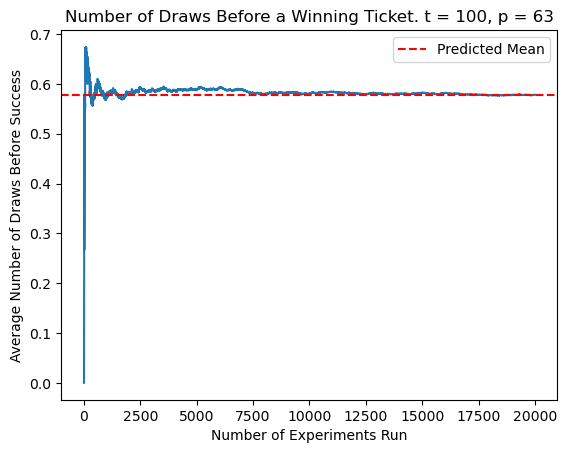
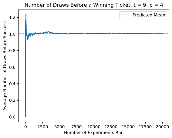
Though the multiple derivations convinced me that my work was correct, I wanted to see it in practice. To do this, I ran simulations using Python. Here, I am finding the number of draws before a winning ticket is found, as I considered in the intuitive solution.
I initialized \(t\) and \(p\) to arbitrary numbers and ran 20,000 trials, tracking the number of draws in every simulation and updating my average. After trying multiple values of \(t\) and \(p\), it was clear from my plots that my formula was correct; the experimental averages indeed converged to my predicted result.
Suppose, for some reason, we want to see both a valid and invalid ticket. Equivalently, say we are drawing balls of two colors out of an urn without replacement and want to see both colors. On average, if we start with \(\boldsymbol{a}\) amber balls and \(\boldsymbol{b}\) brown balls, how many draws without replacement are needed before seeing both colors?
This is actually a simple extension of the last problem. By the holes argument, we expect \(\frac{b}{a+1}\) brown balls to appear before the first amber, and \(\frac{a}{b+1}\) amber balls to appear before the first brown. Since the first ball drawn is always one color or the other, these two expectations add directly - there is no overlap to correct for, and our answer is simply their sum:
Testing the Two Colors Case
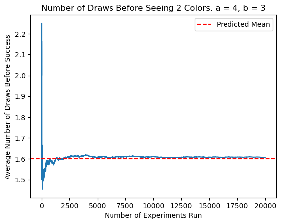
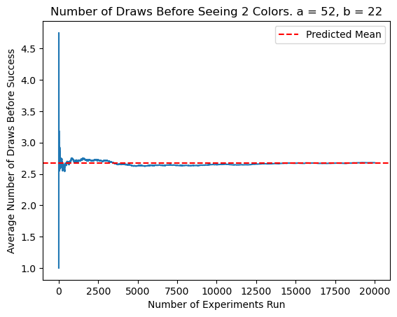
I modified my previous simulation to take in values for \(a\) and \(b\) to determine how many draws are necessary before finding both colors. Once again, the experimental average converged to the results of my expected value calculations.
Now, we have \(\boldsymbol{a}\) amber balls, \(\boldsymbol{b}\) brown balls, and \(\boldsymbol{c}\) cyan balls in an urn. On average, how many draws must be made without replacement before drawing balls of all colors?
This problem was harder to tackle. My instinct was that a quick extension of what I had done in the case of two colors wouldn't work. This time, the last color to appear could not define the entire progression of colors; thus my cases, as I defined them, were no longer mutually exclusive.
I tested my theory experimentally. For \(a\) amber balls, \(b\) brown balls, and \(c\) cyan balls, I tried:
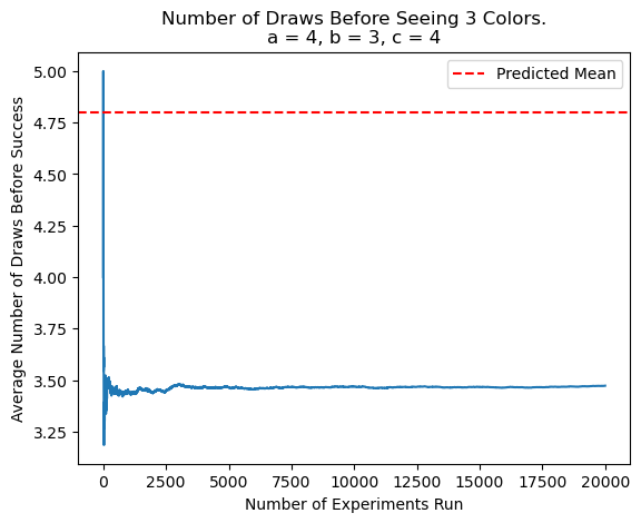
One way to think about it is, regardless of the sequence of colors you draw from the urn, you can reorganize them into three groups: those of the first color seen, those of the second, and the single ball from the third and final color. The sequences don't really matter because we're counting the total number of draws, and on average, we expect a constant number of balls in each group. Let's take the case of an amber ball coming out first or second. From this new perspective, it's clear that the \(\frac{a+b}{c+1} + \frac{a+c}{b+1}\) contribution to our sum is overcounting the expected number of amber balls. If we envision keeping the amber group at the front, it's clear that we overcounted the expected number of amber balls appearing before brown and cyan balls. Quantified, we overcounted by \(\frac{a}{b+c+1}\). Extending this logic to the other colors, we have:
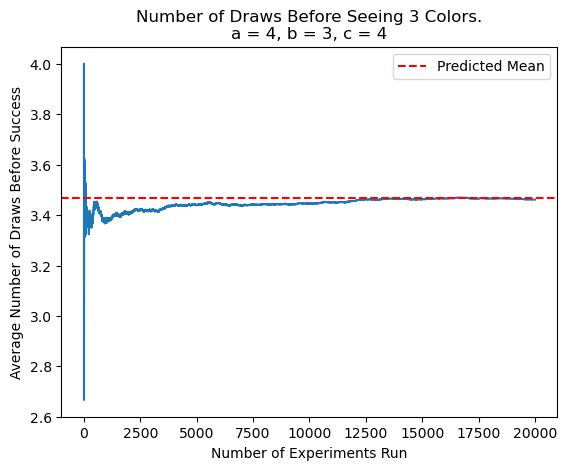
This time, the simulations showed my formula was correct. Indeed, correcting for overcounting by considering one color relative to the other two shifted the expectation down the correct amount.
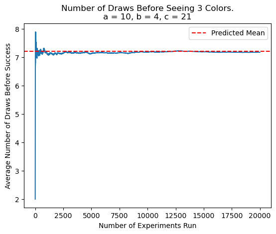
Now, things were getting interesting. I was seeing something like the Principle of Inclusion and Exclusion (PIE) being used in a problem similar to the coupon collector problem. However, rather than drawing from an infinite pool with constant probabilities, here I was drawing from a finite urn. After figuring out the application of PIE in the case of three colors, extending to \(n\) colors wasn't too difficult. Let's state the problem in its extended form:
In an urn, we have balls of \(n\) colors, with a total of \(\sum_{i=1}^{n} b_{i} = B\) balls, where \(b_{i}\) signifies the number of balls of the \(i^{th}\) color. What is the expected number of draws required before seeing all \(n\) colors?
Let \(U = \{1, 2,\dots,n\}\). A straightforward extension of my answer from the cases of two and three colors yielded:
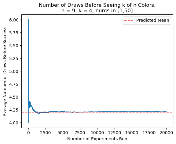
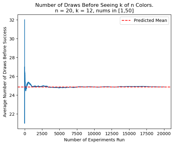
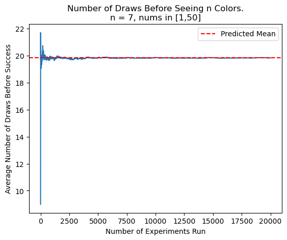
Once again, we see excellent convergence to predicted results. It's worth noting that, due to the exponential time complexity of working with all subsets of \(U\), \(n\) needs to be limited to around 25 or under.
A final challenge to address: We've now found how many draws are needed on average before seeing all \(\boldsymbol{n}\) colors, even with varying the numbers of balls of each color. But now, how do we calculate the expectation of draws before we see \(\boldsymbol{k}\) out of \(\boldsymbol{n}\) distinct colors?
The key insight is to realize that the process of computing this expectation is very similar to any PIE calculation where we calculate the number of elements in at least \(k\) of \(n\) sets, but with a bit of a twist.
First, we need to define some helpful terminology. In the last expectation formula, notice that values are positive or negative depending on the cardinality of \(S\). This is common in PIE calculations, and we can in fact group these partial sums by the cardinalities of \(S\) being considered. For instance, we'll calculate the sum for all subsets \(S\) of length 1, then \(2\), and so on, keeping the absolute values of these quantities. Let's call these values \(v_1\), \(v_2\), etc.
When solving a problem of this "at least \(k\) out of \(n\)" form, the only things that change are the coefficients of each \(v_i\), and the starting point of the alternating sum. As is well known, for this particular PIE problem we always see coefficients of the form:
Thus, we see that when we have \(k=n-1\), we are performing a calculation analogous to computing the number of elements in at least two subsets. Extending this, when we have an arbitrary \(k\), we're finding the number of elements in at least \(n-k+1\) sets. Therefore, our coefficients are of the form:
Further, we see that \(i = |S|\), and the choice of which values are positive and which are negative is dependent upon \(n\), \(k\), and \(|S|\). Together, we have our expected value expression:
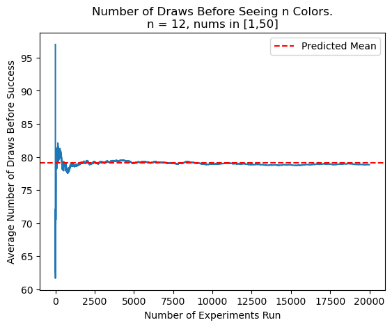
Once again, testing shows that the derived expression works incredibly well to predict the experimental results, i.e., I've found a working solution to the generalized coupon collector without replacement problem.
